Using Excel to Work on Correlation and Regression Examples - Statistics HW Help

For parts 1-8, use the data in the table, which shows the personal income and outlays (both in trillions of dollars) for Americans for 11 recent years.

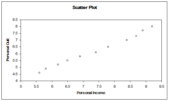
Question 1: Construct a scatter plot for the data. Do the data appear to have a positive linear correlation, a negative correlation, or no linear correlation? Explain.

Solution: The scatter plot is shown in the figure below:

The scatter plot shows a positive correlation. This means that increase in \(x\) is followed by an increase in \(y\).

Solution: Using Excel, we find

This means that the correlation coefficient is equal to:

\[r=0.9959\]

This coefficient is very close to 1, which indicates a very strong (positive) linear association between the variables.

Question 3: Test the level of significance of the correlation coefficient. Use \(\alpha =0.05\)

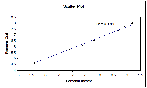
Question 4: Find the equation of the regression line for the data. Include the regression line in the scatter plot.

SUMMARY OUTPUT
Regression Statistics
Multiple R	0.995918
R Square	0.991852
Adjusted R Square	0.990947
Standard Error	0.109835
Observations	11
ANOVA
	df	SS	MS	F	Significance F
Regression	1	13.21688	13.21688	1095.589	1.03E-10
Residual	9	0.108574	0.012064
Total	10	13.32545
	Coefficients	Std. Error	t Stat	P-value	Lower 95%	Upper 95%
Intercept	-0.35871	0.201982	-1.77594	0.109475	-0.81562	0.098207
Personal Income x	0.891226	0.026926	33.09968	1.03E-10	0.830316	0.952136

Solution: We evaluate the regression line at \(x=5.3\) to get

\[\hat{y}=-0.35871+0.891226\times 5.3=4.364789\]

Solution: The coefficient of determination is computed as:

\[{{r}^{2}}={{0.995918}^{2}}=0.991852\]

Solution: Using the Excel table above, the standard error is computed as

\[{{s}_{e}}=\sqrt{\frac{\sum{{{\left( {{Y}_{i}}-{{{\hat{Y}}}_{i}} \right)}^{2}}}}{n-2}}=0.109835\]

The standard error \({{s}_{e}}\) corresponds to an approximation of the standard deviation of the average response. This standard error is very small, which indicates an excellent linear fit.

Solution: First, the point wise prediction is given by:

\[\hat{y}=-0.35871+0.891226\times 6.4=5.345138\]

The 95% prediction interval is given by:

\[CI=\left( \hat{y}-E,\text{ }\hat{y}+E \right)=\left( 5.345138-E,\text{ }5.345138+E \right) \]

where

\[E={{t}_{\alpha /2}}\times {{s}_{e}}\sqrt{\frac{1}{n}+\frac{{{\left( X-\bar{X} \right)}^{2}}}{\sum{{{X}^{2}}-n{{{\bar{X}}}^{2}}}}}=2.262159\times 0.109835\sqrt{\frac{1}{11}+\frac{{{\left( 6.4-7.4 \right)}^{2}}}{619-11\times {{7.4}^{2}}}}=0.096552\]

which means that

\[CI=\left( 5.345138-E,\text{ }5.345138+E \right)=\left( 5.248586,\text{ }5.44169 \right) \]

Question 9: The equation used to predict sunflower yield (in pounds) is

\[\hat{y}=1257-1.34{{x}_{1}}+1.41{{x}_{2}}\]

Solution: We have to replace the given values in the multiple regression equation

(a) \(\hat{y}=1257-1.34\times 2103+1.41\times 2037=1311.15\,\text{ pounds}\)

(b) \(\hat{y}=1257-1.34\times 3387+1.41\times 3009=961.11\,\text{ pounds}\)

(c) \(\hat{y}=1257-1.34\times 2185+1.41\times 1980=1120.9\,\text{ pounds}\)

(d) \(\hat{y}=1257-1.34\times 3485+1.41\times 3404=1386.74\,\text{ pounds}\)

The variable that has more (marginal) effect on the absolute value of the response is \({{x}_{2}}\), because its associated regression coefficient is larger in magnitude.

Question 11: A legal researcher is studying the age distribution of juries by comparing them with the overall age distribution of available jurors. The researcher claims that the jury distribution is different from the overall distribution; that is, there is a noticeable age bias in jury selection in this area. The table shows the number of jurors at a county court in one year and the percent of persons residing in that county, by age. Use the population distribution to find the expected juror frequencies. Test the researcher’s claim at \(\alpha =0.01\).

	21-29	30-39	40-49	50-59	60 and above
Jury	45	128	244	224	359
Population	20.50%	21.70%	18.10%	17.30%	22.40%

Solution: We need to test the null hypothesis:

\[{{H}_{0}}:{{p}_{1}}=0.205,\text{ }{{p}_{2}}=0.217,\text{ }{{p}_{3}}=0.181,\text{ }{{p}_{4}}=0.173,\text{ }{{p}_{5}}=0.224\]

The Chi-Square statistics is computed as:

\[{{\chi }^{2}}=\sum{\frac{{{\left( {{O}_{i}}-{{E}_{i}} \right)}^{2}}}{{{E}_{i}}}}=279.7048\]

The critical value for 4 degrees of freedom, and \(\alpha =0.01\) is

\[\chi _{C}^{2}=13.2767\]

Since \({{\chi }^{2}}>\chi _{C}^{2}\), we reject the null hypothesis, which means that the proportions are not the same as in the population.

Question 14: The table shows the age distribution of a random sample of fatally injured male and female passenger vehicle drivers whose blood alcohol content was at least 0.08 in a recent year. Use \(\alpha =0.05\).

Solution: We’ll use a Chi-Square statistics to test for the independence between Gender and Age Group in terms of the number of accidents involving alcohol consumption. We have the following tables:

Observed Frequencies
	Age Group
Gender	16-20	21-30	31-40	41-50	51-60	61+	Total
Male	155	280	265	225	155	50	1130
Female	60	145	145	130	65	15	560
Total	215	425	410	355	220	65	1690

Expected Frequencies
	Age Group
Gender	16-20	21-30	31-40	41-50	51-60	61+	Total
Male	143.7574	284.1716	274.142	237.3669	147.1006	43.46154	1130
Female	71.2426	140.8284	135.858	117.6331	72.89941	21.53846	560
Total	215	425	410	355	220	65	1690

The Chi-Square statistics is computed as:

\[{{\chi }^{2}}=\sum{\frac{{{\left( {{O}_{ij}}-{{E}_{ij}} \right)}^{2}}}{{{E}_{ij}}}}=9.95144\]

The critical value for 4 degrees of freedom, and \(\alpha =0.05\) is

\[\chi _{C}^{2}=11.07048\]

Since \({{\chi }^{2}}<\chi _{C}^{2}\), we fail to reject the null hypothesis, which means that we don’t have enough evidence to claim that Age Group and Gender are dependent..

In parts 20 and 21, find the critical F-value for a right-tailed test using the indicated level of significance \(\alpha\) and degrees of freedom d.f.N and d.f.D

Solution: We have that \({{F}_{C}}=2.286434\)

Solution: We have that \({{F}_{C}}=2.394025\)

Question 26: A steel pipe fittings company claims that the yield strength of its nontempered couplings is more variable than that of its tempered couplings. A random sample of nine tempered couplings has a standard deviation of 1.31 megapascals, and a similar sample of nine nontempered couplings has a standard deviation of 25.4 megapascals. From past data, it is known that the company’s production process results in normally distributed yield strengths. Test the company’s claim at \(\alpha =0.05\)

Solution: We need to test

\[\begin{array}{cc} &{{H}_{0}}:{{\sigma }_{1}}={{\sigma }_{2}} \\ &{{H}_{A}}:{{\sigma }_{1}}<{{\sigma }_{2}} \\ \end{array}\]

We use an F-test, and the F-statistics is computed as:

\[F=\frac{s_{2}^{2}}{s_{1}^{2}}=\frac{{{25.4}^{2}}}{{{1.31}^{2}}}=375.9455\]

The critical value for d.f.N = 8, d.f.D. = 8, \(\alpha =0.05\) is \({{F}_{C}}=3.438103\). Since \(F>{{F}_{C}}\), we reject the null hypothesis, which means that we have enough evidence to support the claim that the yield strength of its nontempered couplings is more variable than that of its tempered couplings, at the 0.05 significance level.

---

You can send you Excel Stats homework problems for a Free Quote. We will be back shortly (sometimes within minutes) with our very competitive quote. So, it costs you NOTHING to find out how much would it be to get step-by-step solutions to your Stats homework problems.

Our experts can help YOU with your Statistics Assignments. Get your FREE Quote..

Contact Us!