Learn How to Detect and Handle with Multicollinearity in SPSS

The accompanying data set presents simulated financial data of some companies drawn from four different industry sectors. The data include return on capital, sales, operating margin, and debt-to-capital ratio. All the data pertain to the most recent 12 months for which data were available for each company. The specific time period may be different for different companies, but we shall ignore that issue for purposes of data analysis.

Using suitable dummy or indicator variables to represent the sector of each company, regress the return on capital against all other variables, including the indicator variables.

1. Make histograms of each of the four variables. Then do scatter plots among the four variables.

What do the histograms and bivariate plots imply about the computed Pearson correlations among the four variables?

What might you do about possible problems with the correlations or with the resultant multiple regression models?

Solution: Using SPSS we have the following histograms:

RETURN

SALES

MARGIN

DTOC

The data seem to have a reasonable bell shape (except for SALES, which has a strong positive Skewness) to some degree.

Now we present the matrix of scatter plots:

The scatter plots show a rather low degree of linear correlation between the pairs. In fact, we observe the correlation matrix given below:

We see a confirmation of the visual trend of low correlation. But still, the correlation matrix shows that some of the pairs a correlation significantly different form zero (the pairs with the ** in the table).

The correlation between RETURN and the rest of the variables is a desirable correlation. Nevertheless, the correlation between SALES and DTOC and between MARGIN and DTOC is not desirable because it may cause multicollinearity, which is an undesired effect. After running a Multiple Regression we should analyze the VIF indicator to check for signs of collinearity. In that case we might have to drop a variable.

2. The sectors are to be ranked in descending order of return on capital. What will that ranking be?

Solution: First, we use three dummy variables to codify the categorical variable SECTOR. We call these variables:

• BANKS: 1 if the sector is “Banks”, 0 elsewhere.

• COMPUTER: 1 if the sector is “Computers”, 0 elsewhere.

• CONSTRUCT: 1 if the sector is “Construction”, 0 elsewhere.

This way, the sector corresponds to “Energy” when all the previous dummy variables are zero.

On this first stage of the analysis, we analyze the model:

\[\begin{array}{cc} & RETURN={{\beta }_{0}}+{{\beta }_{1}}SALES+{{\beta }_{2}}MARGIN+{{\beta }_{3}}DTOC+{{\beta }_{4}}BANK \\ & \text{ }+{{\beta }_{5}}COMPUTER+{{\beta }_{6}}CONSTRUCT+\varepsilon \\ \end{array}\]

We run a regression analysis using SPSS. The results are shown below:

• We first observe that there are no signs of serious multicollinearity (\(VIF’s < 4\)). Also, we see that the overall model is significant (\(p = 0.000\)).

• We also observe that all the variables are significant, except for BANKS and SALES.

• Also, for the different categories, the higher the$\beta $coefficient, the higher the impact on the RETURN variable. The effects are measured with respect to the “Energy” category. Using that criteria, we have that the descending ranking of the sectors would be

1. Computers
2. Construction
3. Banks
4. Energy

(We have to look “Banks” closely, because the coefficient \({{\beta }_{4}}\) is not significantly different from zero in the regression).

To confirm this result, we run ANOVA to test the mean return for each sector

\[\text{ }{{H}_{0}} :{{\mu }_{BANK}}={{\mu }_{COMPUTERS}}={{\mu }_{CONSTRUCTION}}={{\mu }_{ENERGY}}\]

Results from ANOVA

The results of the ANOVA, together with the Post-Hoc analysis are shown below:

Results from Levene's Test

• The Levene Test shows that we reject the null hypothesis of equal variances.

This shows that we can reject the null hypothesis of equal returns per sector (p = 0.000), so we perform Post-Hoc tests:

According to the table, the order should be

1. Computers

2. Construction

3. Banks

4. Energy

(We cannot say with 95% confidence that “Construction” and “Bank” are significantly different)

3. It is claimed that the sector that a company belongs to does not affect its return on capital. Conduct an appropriate test within multiple regression to see if all the indicator variables can be dropped from the regression model.

Solution: We need to test the following hypotheses:

\[\begin{array}{cc} & {{H}_{0}}:{{\beta }_{4}}={{\beta }_{5}}={{\beta }_{6}}=0 \\ & {{H}_{A}}:\text{ at least on of those }\beta 's\ \text{is not zero} \\ \end{array}\]

As shown before, we have the following table:

This table shows that SALES is not significant for the model (p = 0.333), and BANK is not significant either (p = 0.481).

The rest of the variables are significantly different from zero, and therefore, we reject the null hypothesis. In other words, we have enough evidence to claim that the sector that a company belongs to does affect its return on capital, at the 0.05 significance level.

4. For each of the four sectors, give a 95% prediction interval for the expected return on capital for a company with the following annual data: sales of $3 billion, operating margin of 31%, and a debt-to-capital ratio of 37%.

Solution: We construct the 95% prediction interval for each sector:

• Banks:

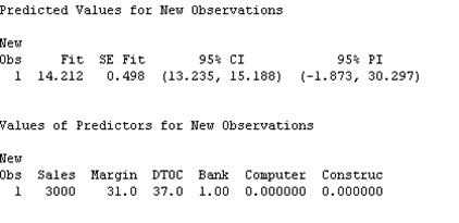
This means that the 95% predicted interval is \((-1.873, 30.297)\).

• Computers:

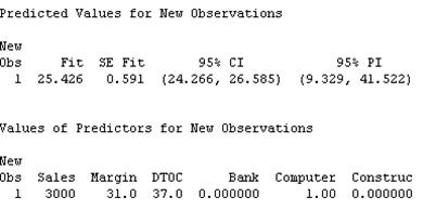
This means that the 95% predicted interval is \((9.329, 41.522)\).

• Construction:

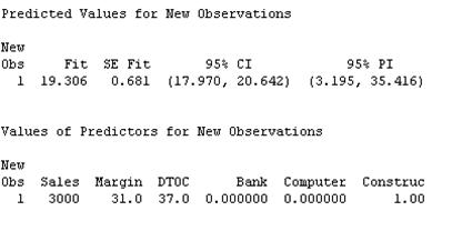
This means that the 95% predicted interval is \((3.195, 35.416)\).

• Energy:

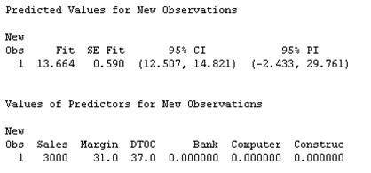
This means that the 95% predicted interval is \((3.195, 35.416)\).

5. Use the three metric (continuous) independent variables and appropriate sector indicator variables to create three possible quadratic independent variables and 18 possible simple two way ANOVA interaction effects among the independent variables and sector classification.

Use the hierarchical multiple regression method to explore whether the quadratic effects or the 18 interaction effects are statistically significant. If you found any significant quadratic or two way interaction effects, how should you interpret them?

Part 2: How to Deal with An Anomalous Data Set in SPSS

Examine the data set called “anomaly.” Y is the dependent variable, and X1 and X2 are the independent variables. Use multiple regression analyses to model Y from X1 and/or X2.

What problems, if any, arise with this data set? What can or should you do to detect and reduce these problems?

Solution: Let’s analyze the variables using histograms and scatter plots:

Now we display the matrix of scatter plots:

• Just by seeing the graph we notice that there’s a very clear linear correlation between the two independent variables. This indicates that most likely we’ll find multicollinearity problems.

Now we run a multiple regression analysis using SPSS. We obtain the following results:

• At first sight it looks like a significant model, with a very high R-square, but there’s a clear multicollinearity problem (VIF’s = 185.529). This means that essentially \({{X}_{1}}\) is a linear function of \({{X}_{2}}\).

One possible way to solve this problem is to drop one of the variables, but this could bring some problems too. If we run the linear regression without the second independent variable we obtain

• The correlation coefficient is not significantly different from zero, and therefore there is not enough evidence of linear association

If we run the linear regression without the first independent variable we obtain

• The correlation coefficient is not significantly different from zero either, and therefore there is not enough evidence of linear association.

CONCLUSION

We need to reformulate the model adding new variables, avoiding multicollinearity.

---

Send us your SPSS homework problems for a Free Quote. We will be back shortly (sometimes within minutes) with our very competitive quote. So, it costs you NOTHING to find out how much would it be to get step-by-step solutions to your Stats homework problems.

Contact Us!