Excel Time Series Forecasting and Regression Analysis - Statistics HW Help

Time Series Forecasting and Regression Analysis

1. The company I work for keeps track of passengers moved on an annual basis. Below are the ride fares for the corresponding years. Forecast the expectation for 2005.

Also, do you think that my company is meeting a community expectation to provide mass transit, is there something more we could do (or less). What do you think about gas prices affecting our ridership in 2005.

Year # of riders (in Millions)

1993 23

1994 28

1995 34

1996 39

1997 35

1998 40

1999 43

2000 45

Solution: Using Excel, we run a Regression Analysis, and obtain the following results

SUMMARY OUTPUT
Regression Statistics
Multiple R	0.945855
R Square	0.894641
Adjusted R Square	0.877081
Standard Error	2.626558
Observations	8
ANOVA
	df	SS	MS	F	Significance F
Regression	1	351.4821	351.4821	50.94823	0.000381
Residual	6	41.39286	6.89881
Total	7	392.875
	Coefficients	Standard Error	t Stat	P-value	Lower 95%	Upper 95%
Intercept	-5739.71	809.1556	-7.09346	0.000394	-7719.65	-3759.78
Year	2.892857	0.405287	7.137803	0.000381	1.901155	3.884559

This means that the model is estimated as

\[Riders=-5,739.71+2.892857\text{ }Year\]

For the year 2005, we have the estimate

\[Riders=-5,739.71+2.892857\times 2005=60.46429\]

This means that the estimate for the ridership in 2005 is 60.46429 million people. Definitely, the ridership is growing in time and that consideration should be taking into account for future expansion of the company in order to meet the future demand.

2. The annual numbers of deer strikes reported with civil aviation (private and commercial are listed below in actual numbers and by year. Predict the number in 2005 and assess concern or lack of concern you have about the numbers.

Year # of Airplanes Striking deer (OF course, on the ground Silly, deer don't fly)

1985 77

1987 82

1989 96

1991 105

1993 121

1995 104

1997 141

1999 129

2001 153

Solution: Using Excel, we find that

SUMMARY OUTPUT
Regression Statistics
Multiple R	0.939361
R Square	0.882399
Adjusted R Square	0.865599
Standard Error	9.512398
Observations	9
ANOVA
	df	SS	MS	F	Significance F
Regression	1	4752.6	4752.6	52.52321	0.00017
Residual	7	633.4	90.48571
Total	8	5386
	Coefficients	Standard Error	t Stat	P-value	Lower 95%	Upper 95%
Intercept	-8756.85	1223.751	-7.15574	0.000184	-11650.6	-5863.14
Year	4.45	0.614023	7.24729	0.00017	2.998068	5.901932

The model corresponds to

\[Deer\text{ }Strikes = -8756.85+4.45\text{ }Year\]

For the year 2005 we get the estimate

\[Deer\text{ }Strikes = -8756.85+4.45\times 2005=165.4\]

This indicates that the number of accidents have an increasing pattern in time, which is very concerning. Something should be done to change that trend.

3. Typical collection of gross sales receipts for a company I used to work for on an annual basis.

Predict 2006 and tell me what you think of the health of the company

Year Sales (in millions)

1995 11

1996 14

1997 12

1998 18

1999 17

2000 24

2001 17

2002 28

Solution: The following table summarizes the regression analysis.

The model is
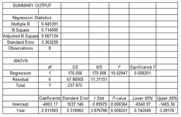
\[Sales=-4003.17+2.011905\text{ }Year\]

For the year 2006 we have

\[Sales=-4003.17+2.011905\times 2006=32.71429\]

This means that the financial health of the company looks very promising from the year 2006

4. Displayed below are the number of alarms that have sounded in the state of Ohio for the last 15 years when dangerous weather has been sighted visually or on radar. Predict the alarms expected in 2006 and tell me if I should consider moving from the state. Why or why not?

Year # weather Alarms

1986 34

1987 43

1988 26

1989 38

1990 45

1991 26

1992 41

1993 28

1994 39

1995 51

1996 47

1997 24

1998 38

1999 42

2000 47

Solution: Excel provides the following output

The model is
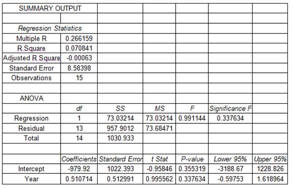
\[Weather\text{ }Alarms=-979.92+0.510714\,Year\]

The predicted value for the year 2006 is

\[Weather\text{ }Alarms = -979.92+0.510714\times 2006 = 44.57262\]

We notice that the p-value of the variable Year is p = 0.337634, which means that the variable is not significant. As a conclusion, there may not be an increasing trend in time of the number of weather alarms every year. Now, that doesn’t mean that the number of weather alarms every year is pretty high in general.

5. My Brother and I own acreage in Wisconsin and since 1980 we have had a small business in Christmas Tree production. It takes 5 years from planting setouts, 2 trims at the beginning of year 3 and 5 to bring the tree to market. My brother and my nephews cut, transport and sell the trees in Hudson Wisconsin. Here are some coded sales (proper ratios from year to year but altered to keep real revenue secret) we have had since 1985. The planting takes 2 partial weeks, each trimming takes 2 partial weeks, the sales requires 2-3 people for 3.5 weeks.

Predict gross sales in dollars for 2005

We are considering whether or not to continue. Give me your opinion based on your analysis

Year Sales (in Dollars)

1985 100

1986 121

1987 133

1988 120

1989 124

1990 120

1991 105

1992 138

1993 140

1994 129

1995 133

1996 140

1997 149

1998 134

1999 160

2000 144

Solution: Here we show the regression analysis

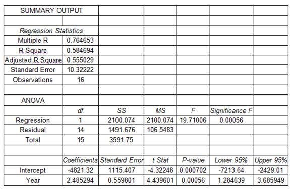
Solution: The model is

\[Sales=-4,821.32+2.485\text{ }Year\]

The estimate for the year 2005 is given by:

\[Sales=-4,821.32+2.485\times 2005=161.6912\]

Most definitely the sales are increasing (the variable Year has significantly positive slope parameter), which means that the business is in good shape. (Obviously we assuming that the profit is also reasonable, or in other words, we are assuming that the cost is not rising as faster than the sales).

6. Here is a company’s years 1990-1996 sales volume per year. Predict the Sales volume for 1999.

Year Sales (in $millions)

1990 12

1991 13

1992 15

1993 14

1994 16

1995 17

1996 19

Solution: The output we get from Excel is

SUMMARY OUTPUT
Regression Statistics
Multiple R	0.960277
R Square	0.922131
Adjusted R Square	0.906557
Standard Error	0.736788
Observations	7
ANOVA
	df	SS	MS	F	Significance F
Regression	1	32.14286	32.14286	59.21053	0.000591
Residual	5	2.714286	0.542857
Total	6	34.85714
	Coefficients	Standard Error	t Stat	P-value	Lower 95%	Upper 95%
Intercept	-2120.21	277.5053	-7.64027	0.000611	-2833.56	-1406.87
Year	1.071429	0.13924	7.694838	0.000591	0.713502	1.429356

The model is given by:

\[Sales =-2,120.21+1,071429\text{ }Year\]

The estimate for 1999 is

\[Sales=-2,120.21+1,071429\times 1999=21.57143\]

7. This is the scrap rate for a company I worked for during the years 1996-2002.

Predict the scrap rate for 2004.

Year Scrap Rate (in final units)

1997 335

1998 299

1999 288

2000 294

2001 204

2002 188

Solution: The regression analysis is shown in the following table:

SUMMARY OUTPUT
Regression Statistics
Multiple R	0.928931
R Square	0.862914
Adjusted R Square	0.828642
Standard Error	24.15308
Observations	6
ANOVA
	df	SS	MS	F	Significance F
Regression	1	14688.51	14688.51	25.17867	0.007397
Residual	4	2333.486	583.3714
Total	5	17022
	Coefficients	Standard Error	t Stat	P-value	Lower 95%	Upper 95%
Intercept	58196.37	11544.5	5.041047	0.007277	26143.64	90249.11
Year	-28.9714	5.773691	-5.01783	0.007397	-45.0018	-12.9411

The regression model is given by

\[Scrap\text{ }Rate=58,196.37-28.9714\text{ }Year\]

The estimate for 2004 is

\[Scrap\text{ }Rate=58,196.37-28.9714\times 2004=137.6286$=\]

8. In 1982 The US Corps of Engineers published this information to the members of the Upper Mississippi Waterways Towing Association. It took the years 1974- 1980 and represented tons of grain to the Gulf by Barge. They then provided a prediction for 1985.

Reproduce the prediction and tell me what could be Wrong with the prediction. When you answer this remember all the droughts, bug infestations, and other phenomena associated with Growing grain affected the data. You have to find something that is another independent variable not captured in the study

1974 24

1975 31

1976 34

1977 39

1978 42

1979 47

1980 53

Solution: The analysis we obtain with Excel is

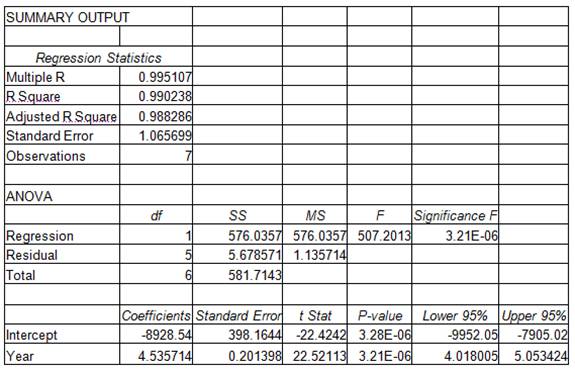
This means that the linear regression model is given by

\[Tons\text{ }of\text{ }Grain=-8,928.54+4.5357\text{ }Year\]

For the year 1985, the prediction would be

\[Tons\text{ }of\text{ }Grain=-8,928.54+4.5357\times 1985=74.85714\]

There are many things that can affect the data in terms of making an estimate not reliable. The conditions when the data were obtained may be not applicable in the future (1985)

9. The car theft rate in the City of Cleveland is displayed in column 2 for the years 1995-2001 forecast the rate for 2002, 2003 and assess the OVERALL safety factor of living in Cleveland

Year Car Theft Rate

1995 1245

1996 1453

1997 1176

1998 1019

1999 945

2000 1001

2001 899

Solution: The output from Excel is shown below:

The model is
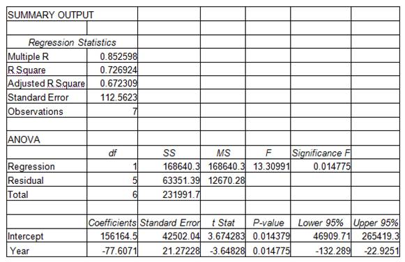
\[Car\text{ }Theft\text{ }Rate=15,164.5-77.6071\text{ }Year\]

v For year 2001 we have

\[Car\text{ }Theft\text{ }Rate=15,164.5-77.6071\times 2001=872.6071\]

v For year 2002 we have

\[Car\text{ }Theft\text{ }Rate=15,164.5-77.6071\times 2002=795\]

v For year 2003 we have

\[Car\text{ }Theft\text{ }Rate=15,164.5-77.6071\times 2003=717.3929\]

This shows that the car theft rate is expected to decrease in the upcoming years, which is a good sign in terms of the overall safety.

---

You can send you Excel Stats homework problems for a Free Quote. We will be back shortly (sometimes within minutes) with our very competitive quote. So, it costs you NOTHING to find out how much would it be to get step-by-step solutions to your Stats homework problems.

Our experts can help YOU with your Statistics Assignments. Get your FREE Quote..

Contact Us!