All the Steps Needed for Model Building and Residual Analysis with the Aid of Minitab

Alan Green, an analyst with Pilgrim Bank, needs to prepare a report for his boss, Ravi Raman, on whether customers who use on-line banking are more profitable, and if adoption of on-line banking by customers makes them more profitable. To prepare analyses to support his report, Alan has obtained data for a random sample of 5,000 customers for both 1999 and 2000. Alan has discovered that there was not a statistically significant difference in mean customer profitability for on-line and off-line customers in 1999, but has a feeling there may be more information that could help Raman decide how to manage customer profitability. To help him determine what that information is, Alan has asked for your help in answering these questions.

a) Why is there a need to predict future customer profitability? In other words, if Pilgrim Bank knows how profitable a customer is today, why do they need to worry about how profitable that customer is tomorrow?

b) Is there a significant difference in 2000 profitability for customers for whom age and/or income data is missing and for customers for whom that data is not missing? Should age and/or income be included as independent variable(s) in a multiple regression model to predict customer profitability in 2000, and why or why not? HINT: This question cannot be answered using regression; you need to use a different tool.

c) Does geographic region predict customer profitability in 2000? Should geographic region be included as an independent variable in a multiple regression model to predict customer profitability in 2000, and why or why not?

d) Does tenure with the bank predict customer profitability in 2000? Should tenure be included as an independent variable in a multiple regression model to predict customer profitability in 2000, and why or why not?

e) How well does customer profitability in 1999 predict customer profitability in 2000? Should customer profitability in 1999 be included as an independent variable in a multiple regression model to predict customer profitability in 2000, and why or why not?

f) How well does the use of on-line banking in 1999 predict customer profitability in 2000? Should on-line banking be included as an independent variable in a multiple regression model to predict customer profitability in 2000, and why or why not?

g) Are there any other variables included in the data set that can help predict customer profitability in 2000?

h) What is the best regression model for predicting customer profitability in 2000, and why?

i) How many customers in Alan’s sample left the bank from 1999 to 2000?

j) What implications do all of these analyses have for the strategies Pilgrim Bank might consider using to manage customer profitability? Write a memo to Alan that provides information to help answer these questions, and include relevant analyses as exhibits (at a minimum include an exhibit with the regression model identified as the best). Be sure to specifically answer questions a) and j) in your memo and describe to Alan how you decided what variables to include in the regression model you found to be the best.

Solution: It is reasonable to think that customer profitability changes in time. Clients can have a bad experience with the bank and withdraw investments, or simply quit. There is a competitive market for banks out there; therefore customers have to be monitored closely.

In addition, new services like online banking, online bill-pay, etc, can entice the customers to do more business with the bank, which in the end will reflect in higher customer profitability. The process of adoption of new technologies can take a fair amount of time which implies changes in customer patterns from year to year. This suggests that even if we know that there was not a statistically significant difference in mean customer profitability for on-line and off-line customers in 1999, it can change during the next year, or even during the next month

Age and/or Income Missing

First of all, we need to create a new table with the 2000 profitability for customers for whom age and/or income data is missing and for customers for whom that data is not missing. We have added a new worksheet to the Excel file with the data.

In order to perform the calculation, we need to apply a t-test to the following hypotheses:

\[\begin{array}{cc} & {{H}_{0}}:{{\mu }_{1}}\le {{\mu }_{2}} \\ & {{H}_{A}}:{{\mu }_{1}}>{{\mu }_{2}} \\ \end{array} \]

where \(\mu_1\) represents the population mean customer profitability (for the year 2000) for clients with known age and income, and \({{\mu }_{2}}\) represents the population mean customer profitability (for the year 2000) for clients with missing age and/or income

Before running the t-test, we need to check whether we can assume equal variances or not. In order to do so, we use an F-test. With the aid of Excel we get the following results

The p-value, as reported in the table, is equal to \(p < .001\), which is less than the significance level \(\alpha = 0.05\). That means that we can assume unequal variances.

Now we perform a t-test for unequal variances. This is the output we obtain from Excel:

The p-value for the one-tailed test is equal to \(p = .036328 < .05\), which means that we have enough evidence to claim that the 2000 profitability for customers for whom age and/or income data is missing is less than for customers for whom that data is not missing, at least at the 0.05 significance level.

Multiple Regression Model

Now, we are going to analyze the significance of the variables in the multiple regression model. We need to prepare the data before attempting a regression though. First, we need to use dummy variables for all the categorical variables, in this case, Age, Income and Geographical Region.

The dummy variables we introduce are called:

• 9Age_d1, 9Age_d2, 9Age_d3, 9Age_d4, 9Age_d5, 9Age_d6 (we need 6 dummy variables for 7 age categories)

• 9Inc_d1, 9Inc_d2, 9Inc_d3, 9Inc_d4, 9Inc_d4, 9Inc_d5, 9Inc_d6, 9Inc_d7, 9Inc_d8 (we need 8 dummy variables for 9 income categories)

• 9district_d1, 9district_d2 (we need 2 dummy variables for 3 geographical regions)

First we run a “naive” regression with all the variables included. Excel only runs multiple regression up to 16 predictors, so we are going to use Minitab instead. The result from the regression will tell us what variables are significant and aren’t.

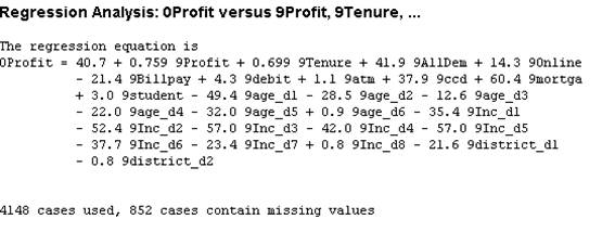
• The following is the ANOVA analysis:

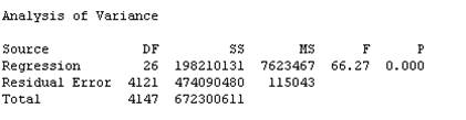
The p-value is equal to \(p < .001\), which means that the model is significant overall. In other words, not all the regression coefficients are equal to zero.

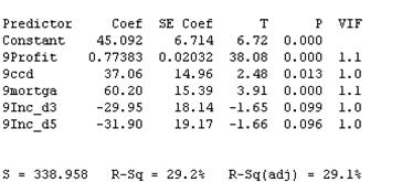
• Now proceed to test the significance of the predictors included in the model:

\[S = 339.179 R-Sq = 29.5% R-Sq(adj) = 29.0%\]

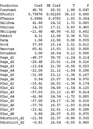
The way we interpret this table is simple: The p-value column represents the significance of the respective predictor. If \(p < .005\), then the predictor is statistically significant. If \(p > .05\), then the predictor is not significant.

From this information we conclude that the variables that are significant are

• 9Profit, 9ccd, 9mortga, 9Inc_d3, 9Inc_d5 (This means that Income is a significant variable)

• The rest of the variables are not statistically significant

Let’s analyze the residuals to verify the integrity of the model.

• We observe a lack of normality of residuals, and some degree of lack of homogeneity in the residuals.

Best Regression Model

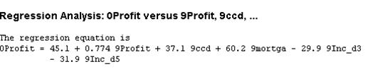
Let’s run the regression with the variables that are statistically significant.

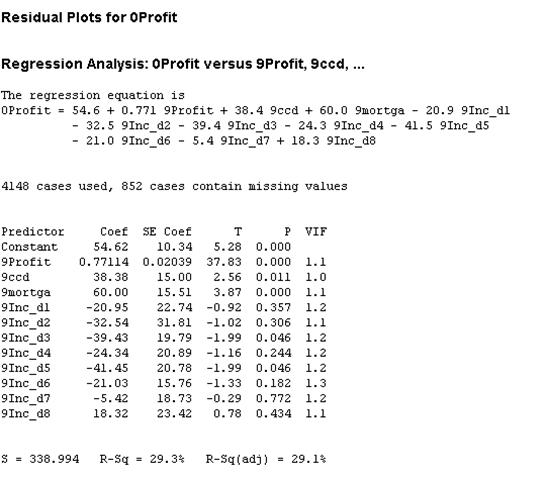
We observe that the Adjusted R-Square increases 0.1% with respect to the model with all the variables. Looking at the p-value column we notice that 9Profit, 9ccd, 9mortga, 9Inc_d3 and 9Inc_d5 are significant (This means that Income is significant).

• Minitab has a very powerful tool called “Best Subsets” which suggests the best model out of the whole set of variables.

The criteria to select model is to include only significant variables if possible, and maximize the Adjusted R-Square. The regular R-Square gets artificially “inflated” by the number of variables, and it’s better to maximize the former.

Minitab uses an automatic algorithm to test all possible models and to select the best models that satisfied the mentioned criteria. But in this issue it’s not black and white only, there’s gray, and a lot of shades of gray. The decision of the ultimate “best model” depends on the knowledge of the analyst, who needs to use her expert eye to put all the elements together and make a decision which is not entire rigidly based on the outcome of the algorithm.

Here we show the results of the Best Models algorithm: We fix “9Profit” in the model, and the rest of the variables are tested to see their contribution to the model.

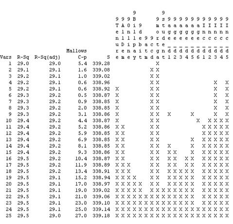
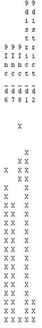
The analysis shows similar Adjusted R-Squared for most of the models, but it seems that the best models that balance maximum Adjusted R-Square, Minimum S, low Mallows C-p and minimum number of variables are:

• The model with 5 variables: 9Profit, 9ccd, 9mortga, 9Inc_d3, 9Inc_d5

The problem with this is that the p-value for 9Inc_d3 and 9Inc_d5 is not significant.

• The model with 3 variables: 9Profit, 9ccd, 9mortga:

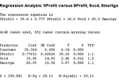
Between these two model we should choose the best one. Considering that the p-value for 9Inc_d3 and 9Inc_d5 is still low (less than 0.1) and that the first model has a smaller S, we choose the model with the 5 variables, but at this point an expert should use her expertise to include Income or not in the model.

Conclusions from Minitab's Bets Subsets

• 852 clients left the bank in 2000.

• The variables that are clearly significant and should definitely be included in the model are 9Profit, 9ccd, 9mortga.

• Income appears to have a significant role in predicting 0Profit, but it depends of the significance we choose.

• The rest of the variables don’t appear to have influence in the dependent variable.

• The overall fit is not too good. Only 29.1% of the variation in 0Profit is explained by the predictors. This suggests to look for more meaningful predictors, or to look a model other than linear.

• The best model is written as

\[0\text{Profit}=39.4+0.777\times 9\text{Profit}+36.0\times \text{9ccd}+60.9\times 9\text{mortga}\]

• Pilgrim Bank should increase and diverse its efforts in those areas that affect customer profitability, like expand its credit card and mortgage operations.

---

Do you have any Minitab questions? Send us your Minitab problems for a Free Quote. We will be back shortly with our very competitive quote. So, it costs you NOTHING to find out how much would it be to get step-by-step solutions to your Stats homework problems.

Contact Us!